Simple Derivative

Suppose we want to differentiate the function \(f(x) = x^2\). For this function we can easily state its analytical derivative \(f'(x) = 2x\).

Instead of implementing the analytical derivative by hand, we want to have it computed algorithmically. Let’s say we are interested in the function value \(f(x)\) and its derivative at \(x=0.5\).

First we need to implement a function f which computes \(f(x)\). We are already able to compute \(f(0.5)\).

def f(x):
    return x**2

print ("f(0.5) = {}".format(f(0.5)));

f(0.5) = 0.25

To generate a function which computes the derivative, we use the derivative function from the pyADiff package. This returns a function for the derivative which we here call df. Now we are able to compute \(f'(0.5)\)

import pyADiff
df = pyADiff.derivative(f)

print("f'(0.5) = {}".format(df(0.5)));

f'(0.5) = 1.0

This result can be verified using the analytical derivative \(f'(0.5) = 2 \times 0.5 = 1\).

It might be more convenient to see the functions \(f\) and \(f'\) as graphs. Therefore the packages numpy and matplotlib.pyplot are included.

import numpy as np
import matplotlib.pyplot as plt

Now we initialize x as 100 points between -1 and 1. And calculate the function value \(f\) and its derivative \(f'\) at each of the points in x. Note the wayf and df are called repeatedly. While for f the numpy vectorization would work as expected and would return all of the inputs x squared, pyADiff would interpret f as a function \(f : \mathbb{R}^{100} \to \mathbb{R}^{100}\), where \(f_i(x) = x_i^2\) and would return the jacobian of \(f\).

Therefore we explicitly call f and df for each x_i in a loop here.

x = np.linspace(-1, 1, 100)

y = np.array([f(x_i) for x_i in x])
dy = np.array([df(x_i) for x_i in x])

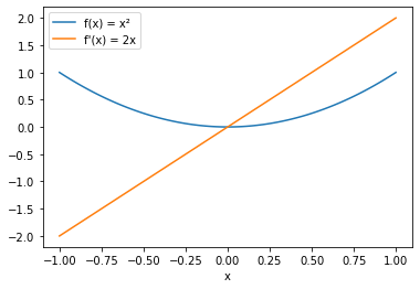
The last step is to plot the function \(f\) and its derivative \(f'\) over x.

plt.plot(x, y, label="f(x) = x²")
plt.plot(x, dy, label="f'(x) = 2x")
plt.xlabel('x')
plt.legend();